BASIC MATRIX OPERATION IN MATLAB

AIM:

          To understand the fundamentals matrix operations carried out in matlab

THEORY:

          The MATLAB@ high-performance language for technical computing integrates computation, visualization, and programming in an easy-to-use environment where problems and solutions are expressed in familiar mathematical notation. Typical uses include

* Math and computation

* Algorithm development

* Data acquisition

* Modeling, simulation, and prototyping

* Data analysis, exploration, and visualization

* Scientific and engineering graphics

          Application development, including graphical user interface building MATLAB is an interactive system whose basic data element is an array that does not require dimensioning. It allows you to solve many technical computing problems, especially those with matrix and vector formulations, in a fraction of the time it would take to write a program in a scalar non interactive language such as C or Fortran.

Role of Simulation in Design

          Electrical power systems are combinations of electrical circuits and electromechanical devices like motors and generators. Engineers working in this discipline are constantly improving the performance of the systems. Requirements for drastically increased efficiency have forced power system designers to use power electronic devices and sophisticated control system concepts that tax traditional analysis tools and techniques. Further complicating the analyst's role is the fact that the system is often so nonlinear that the only way to understand it is through simulation.       

          Land-based power generation from hydroelectric, steam, or other devices is not the only use of power systems. A common attribute of these systems is their use of power electronics and control systems to achieve their performance objectives. Sim Power Systems software is a modem design tool that allows scientists and engineers to rapidly and easily build models that simulate power systems. It uses the Simulink environment, allowing you to build a model using simple click and drag procedures. Not only can you draw the circuit topology rapidly, but your analysis of the circuit can include its interactions with mechanical, thermal, control, and other disciplines. This is possible because all the electrical parts of the simulation interact with the extensive Simulink modeling library. Since Simulink uses the MATLAB@ computational engine, designers can also use MATLAB toolboxes and Simulink block sets. SimPowerSystems software belongs to the Physical Modeling product family and uses similar block and connection line interface.

Invoking MATLAB

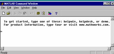
 If MATLAB is successfully installed in the Window platform, an icon is created for it and a folder will be opened for it in Programs folder at the startup. Matlab can be started either by double clicking icon or by selecting the Matlab button from the programs at the startup. Once executed, MATLAB clears the screen, it provides some introductory comments and then generators MATLAB ‘prompt’. The prompt looks like’>>’. Any command in the MATLAB is executed at the prompt. The files of the MATLAB can be edited and stored using any text editor. By default, MATLAB uses Note pad of Windows and note that the files of MATLAB will/should have an extension of .m e.g. ‘Convert.m’. The toolboxes are located in the subdirectory ‘toolbox’ within the MATLAB directory. The path for all the toolboxes is given in the ‘matlabc.m’. Which will be executed by MATLAB at the time of invoking it. Just after invoking MATLAB, the screen looks like the one below.

Working with MATLAB

It is very simple to work in MATLAB environment as most of the commands are entered as they are written mathematically. For example, at the prompt the following command (expression)

                        >>k = 10/3

                        given the output as

                        k = 3.3333

and assigns the value 3.3333 to the variable k. In commands after this command k can be used as it is defined with a value just now. MATLAB recognizes first 19 characters of a variable name and requires only the first character in a variable name be a letter. Like C/C++, MATLAB is also case sensitive in the sense that the variable ‘a’ and ‘A’ are different and can be used in a single file/command with different values. ALL MATLAB commands are written in lower case letters. The arithmetical computations without using variables are also permitted. For example

>> 10 + 5/3

gives the output as

ans =

            11.6667

This computed value is stored in the variable ‘ans’ and can be used letter as long as it is note modified with the computations like above. Blanks (white spaces) can introduce in the commands so that readability is enchanced. If the command is wrongly typed or the syntax is wrong, then the output will be an error message, normally indicating the type of error in the command. MATLAB responds with reasonably understandable statements in case of computations resulting in zero in the denominator, zero divided by zero and infinity by infinity etc.

The following are some examples for computations that can be done in MATLAB.

Programming in MATLAB

The objective of the first program is – Two numbers are taken as input and then their sum is printed out as output.

Invoke Matlab. Select ‘File’ then the select ‘New’ from it and then ‘M-file’. Windows wordpad is automatically opened. Enter the following text and then save it as ‘first.m’.

                                    a = input (‘Enter the value of a’)

                                    b = input (‘Enter the value of b’)

                                    c = a+b

Then at the command prompt just type ‘first’. Then MATLAB prompts for the value of a with the string ‘Enter the value of a’, for the first statement. Respond with a value 4. For the second statement, MATLAB prompts for the value of b with the string ‘Enter the value of b’ Respond with a value 5. Then output will be given as c=9.

The file ‘first.m’ can be executed again by simply typing ‘first’ at the command prompt. Now, give the values as 5 for a and (5*a) fir B. Then the output will be c =30. Note that the value (5*a) is a valid MATLAB expression as A is just defined in the previous statement. The command ‘input’ prints out the text given in it and then waits for the input from the keyboard. Execute the same file again and give values as ‘3+4i’ for a and ‘5+2i’ for b. See the output, it will be c = 8+6i, which means the variables of MATLAB are not having any restrictions on their type, like the variables of other programming languages. E.g C language requires variables to be declared first with their type., like ‘int’ or ‘float’. Then the variables, which are declared at ‘int’ type, cannot be assigned with the values like 10.62 etc. MATLAB has no such limitations, which makes it extremely simple.

Formatting the output

The statement ‘FORMAT’ sets the way any output is printed. It may noted that all computations in MATLAB are done in double precision. FORMAT statement may be used to switch between different the use of FORMAT statement

^aThe data value used for the example is 12.345678901234567 in all cases.

CONTROL STATEMENTS IN MATLAB

IF Statement

IF Conditionally execute statements. The general form of an IF statement is : IF variable, statements, END. For example

k=8;i=1;j=1;a=1;b=2;

if k==10

   c=2

 elseif a==8

        a(i,j)=-1

     else

       a(i,j)=0

end

FOR STATEMENT

Repeat statements a specific number of times. The general form of a FOR statements is ;

FOR variable = expr, statement …, Statement END

The columns of the expression are stored one at a time in the variable and then the following statements, up to the END, are executed. The expression is often of the form X:Y, in which case its columns are simply scalars.  The example below illustrates the use of FOR loop. The objective is to find the sum of all the elements in a vector ‘x’. Then find a vector ‘z’ as a sun of two vector ‘x’and’y’.

x=0:1:10;

y=[-1 2 40 2 4 8 9 1 5 3 7];

lv=length(x);

sum=0;

for k=1:lv

   sum=sum+y(k);

   z(k)=x(k)+y(k);

end

sum

 The first line begins with the symbol % indicating a comment. In other words, a statement beginning with % symbol will not executed by MATLAB. The line x= 0:1:10; defines an array \ vector ‘x’ with elements beginning with zero (first element) and ending at 10 (last element) with an increment 1. The semicolon at the end of the statement is stop the printing of output of that statement to the screen , if semi – colon is absent, the vector ‘x’ would  have been printed on the screen immediately after the statement is executed. Next statement y=[-1 2 40 2 4 8 9 1 5 3 7 ]; is the definition of the vector ‘y’ with its actual elements. Observe that the elements in a vector are separated by blanks. Commas can also be used in between the element the elemental values to enhance the readability.

 That is, the two statement y=[-1 2 40 2 4 8 9 1 5 3 7 ]; and y=[-1,2,40,2,4,8,9,1,5 , 7 ]; are one and the same. Another way of defining a vector is to use the statement ‘fscanf’ and ‘fread’. For that matter, vectors can be defined using the statement ‘ones’, ‘zeros’ and ‘size’. The next statement defines the variable lv as the length of vector ‘x’ though, the no of elements (or size) of ‘x’ is known here in this example. This way of writing program for finding the length of vectors eliminates any possible errors in further manipulations. Next, the ‘FOR’ loop is initialized. It starts at I and terminates at the value of lv, which is the size of the vectors ‘x’. Here, no step is mentioned and hence the MATLAB assumes the default step which is l .The end of the for loop is indicated by ‘end’. Finally the simple statement ‘sum’ is to print the value of the variable sum on to the screen.

 However, for finding the sum of the elements of a vector a separate program like the one above need not be written. MATLAB has a built in function ‘sum’ for the same purpose. Use the function in the above program, keeping the original code as it is. Observe that MATLAB gives errors message. Why ?

WHILE STATEMENT

Repeats statements an indefinite number of times. The general from of a WHILE statement is: WHILE variable, statements, -----, statement, END

 The statement are executed while the while the variable has all non – zero elements.

k=0;

i=1;

sum=0;

x=[0 1 2 3 4 5 6 7 8 9 10];

while k<10

   sum = sum+x(i);

   i=i+1;

   k=k+1;

end

sum

Matrices in MATLAB   

Row and column vectors can be defined as below. 

           a= [1 2 3 4 5]

          a =

     1  2   3  4  5

>> b= [1; 2; 3; 4; 5]

b =

1

2

3

4

5

Semi column indicates the end of row. A row vector can be converted in to a column vector by transposing it. The command for transposing a matrix is a’. for example,

 >> k =[- 2 3 4 ]

k=

    -2  3  4

>> k’

ans =

-2

3

4 

The statement  I= 0:1:10 generates a column vector of 11 elements, starting at 0 and ending at 10 with a step of 1.

Two and three dimensional plotting   

MATLAB can create high resolution, publication quality two and three dimensional, linear, semilog, log, polar, bar chart and contour plots on plotters, dot – matrix printers and laser printers. These graph windows can be latter copied on to clip – board or as a windows meta file.

  Solution of Differential Equations  

 MATLAB provides two functions for numerical solution of differential equations employing the Runga –Kutta method. These are ode23 and ode45, based on the Fehlberg – second and third – order pair of formulae for medium accuracy and fourth – and fifth – order pair for higher accuracy. The nth order differential equations must be transformed into n first order simultaneous differential equations and must be placed in an M – file that returns the state derivatives of the equations.

String operations 

 A sequence of characters in single quotes is call a character string or text variable.

c= ‘Good’ results in c= Good

A text variable can be augmented with more text variables, example

cs = [c, ‘luck’ ] produces cs = Good luck

File  I/O

The MATLAB command FOPEN is used for opening a file.

FID = FOPEN (‘filename’, permission) opens the specified file with the specified permission.

Permission is one of the strings:

                    ‘r’            read

                    ‘w’           write (create if necessary)

                    ‘a’            append (create if necessary)

                    ‘r +’         read and write (do not create)

                    ‘w +’        truncate or create for read and write

                    ‘a +’         read and append  (create if necessary)

                    ‘W’          write without automatic flushing

                    ‘A’           append without automatic flushing

By default, files are opened  in binary mode. To open a text file, add ‘t’ to the permission string, for example ‘rt’ and ‘wt+’, (on Unix and Macitosh systems, text and binary files are the same so this has no effect. But on PC and VMS systems this is critical.) The statement FID = FOPEN (‘filename’) assumes a permission fo ‘r’. if the file is open in ‘r’ mode and it is not found in the current working directory, FOPEN searches down MATLAB’s search path.

The commend FCLOSE(FID) closes the file with file identifier FID, which is an integer obtained from earlier FOPEN ( ). FCLOSED (‘all’) closed all open files.

The most important function is FPRINTF. It is used to write formatted data to file. The MATLAB statement NBYTE = FPRINTF (FID, FORMAT, A,------) formats the data is matrix A, under control of the specified FORMAT string, and writes it to the file associated with file identifier FID. NBYTE is an optional output argument that returns the number of bytes, if successfully written.

FORMAT is a string containing C language conversion specifications. Conversion specifications involve the character % optional flags, optional width and precision fields, optional subtype specified, and conversion characters d, i, o, u, x, X, f, E, g, G, c, and s.

Using On – line Help of MATLAB 

An excellent online help is available in MATLAB. Help can be obtained by the key word ‘help’ For example, help on the command ‘format’ can be obtained using ‘help format’.

BUILT – IN FUNCTION OF MATLAB         

 The power of MATLAB comes from its built in library functions. These functions help programmers in simulating the systems easily. Simulation of physical systems is nothing but the true translation of systems or its dynamics into mathematical equations and then solving them. These equations could be simple algebraic equations, or matrix equations, or differential equations or simultaneous differential equations. If these equations are ‘characteristic equations’ of the systems, then their solution will give the state of affairs of the   system at a given instant.  For solving the equations of the kind above, several lines of code has to be written.  Then the programmer or the person who model the system requires an extensive knowledge of mathematics apart from the system.  Fortunately, packages like MATLAB cut down the burden of writing code for such tasks.  For example, to arrange an array in ascending order, one of the standard techniques like bubble sort, or quick sort has to be taken then code has to be written.  Generally built in libraries of prevailing programming languages support only basic functions like, SIN, COS, ABS.. etc., and do not host any ready-made functions for sorting, or matrix inverse etc. The biggest advantage with MATLAB is it has ready made functions available with it, which can be used at any part of the code, even they can be modified according to the requirement.  In addition to this user can add his own functions to his libraries or toolboxes.  Some of the built in functions of MATLAB, which are useful and frequently used, are given on table below.

   Special variables:

SOME USEFUL COMMANDS

The command described below, are very useful in MATLAB environment.  They help the users in getting online help, locating the files etc. The commands can also be used in programming.

Operators and special character.

In addition to the above, MATLAB provides over 50 demos for explaining the basic and advanced features of MATLAB.  A complete list of MATLAB demos can be obtained using the command ‘help demons’.

Z =zeros(2,4)

z=

0        0        0        0

0        0        0        0

F =5*ones(3,3)

F=

5 5 5

5 5 5

5 5 5

N = iJX(10*rand(I,10))

N=

9        2        6       4       8       7       4       0       8       4

R =randn(4,4)

R=

0.6353 0.0860 -0.3210 -1.2316

-0.6014 -2.0046 1.2366 1.0556

0.5512 -0.4931 -0.6313 -0.1132

-1.0998 0.4620 -2.3252 0.3792

A = [16.0     5.0     9.0     4.0

          3.0     10.0   6.0     15.0  

          2.0     13.0   11.0   8.0

          7.0     12.0   14.0 1.0 ];

Concatenation is the process of joining small matrices to make bigger ones. In fact, you made your first matrix by concatenating its individual elements. The pair of square brackets, [], is the concatenation operator. For an example, start with the 4-by-4 magic square, A, and form

B = [A A+32; A+48 A+16]

The result is an 8-by-8 matrix, obtained by joining the four submatrices:

B=

16 3 2 13 48 35 34 45

5 10 11 8 37 42 43 40

9 6 7 12 41 38 39 44

4 15 14 1 36 47 46 33

64 51 50 61 32 19 18 29

53 58 59 56 21 26 27 24

57 54 55 60 25 22 23 28

52 63 62 49 20 31 30 17

          This matrix is halfway to being another magic square. Its elements are a rearrangement of the integers 1:64. Its column sums are the correct value for an 8-by-8 magic square:

sum(B)

ans =

260    260    260    260    260    260    260    260

Deleting a row or column

You can delete rows and columns from a matrix using just a pair of square brackets. Start with

X =A;

Then, to delete the second column of X, use

X(:,2) =[]

This changes X to

X=

16      2       13

5        11      8

9        7        12

4        14      1

If you delete a single element from a matrix, the result is not a matrix anymore. So, expressions like

X(I,2) =[]

result in an error. However, using a single subscript deletes a single element, or sequence of elements, and reshapes the remaining elements into a row vector. So

X(2:2: 10) = []

results in

x=

16      9        2       7       13     12     1

Durer's magic square

A = [16        3        2        13

          5        10      11     8

          9        6        7       12

          4        15      14     1 ]

provides several examples that give a taste of MATLAB@ matrix operations. You have already seen the matrix transpose, A'. Adding a matrix to its transpose produces a symmetric matrix:

A+A'

ans =

32      8        11      17

8        20      17      23

11      17      14      26

17      23      26      2

The multiplication symbol, *, denotes the matrix multiplication involving inner products between rows and columns. Multiplying the transpose of a matrix by the original matrix also produces a symmetric matrix:

A'*A

ans =

378    212    206    360

212    370    368    206

206    368    370    212

360    206    212    378

The determinant of this particular matrix happens to be zero, indicating that the matrix is singular:

d = det(A)

d=0

The reduced row echelon form of A is not the identity:

R = rref(A)

R=

1        0        0        1

0        1        0        -3

0        0        1        3

0        0        0        0

Since the matrix is singular, it does not have an inverse. If you try to compute the inverse with

x = inv(A)

you will get a warning message:

Warning: Matrix is close to singular or badly scaled.

Results may be inaccurate. RCOND = 9.796086e-018.

Roundoff error has prevented the matrix inversion algorithm from detecting exact singularity. But the value of rcond, which stands for reciprocal condition estimate, is on the order of eps, the floating-point relative precision, so the computed inverse is unlikely to be of much use.

The eigen values of the magic square are interesting:

e = eig(A)

e=

34.0000

8.0000

0.0000

-8.0000

One of the eigenvalues is zero, which is another consequence of singularity. The largest eigenvalue is 34, the magic sum. That is because the vector of all ones is an eigenvector:

v = ones(4,1)

v=

1

1

1

1

A*v

ans =

34

34

34

34

When a magic square is scaled by its magic sum,

          P = A/34

the result is a doubly stochastic matrix whose row and column sums are

all 1:

          p=

0.4 706        0.0882        0.0588         0.3824

0.1471         0.2941         0.3235         0.2353

0.2647         0.1765         0.2059         0.3529

                   0.1176         0.4412         0.4118         0.0294

Such matrices represent the transition probabilities in a Markov process. . Repeated powers of the matrix represent repeated steps of the process. For our example, the fifth power

          P^5 is

0.2507         0.2495         0.2494         0.2504

0.2497         0.2501         0.2502         0.2500

0.2500         0.2498         0.2499         0.2503

0.2496         0.2506         0.2505         0.2493

poly(A)

          are 1 -34     -64     2176 0

The constant term is zero, because the matrix is singular, and the coefficient of the cubic term is -34, because the matrix is magic!

Arrays

When they are taken away from the world of linear algebra, matrices become two-dimensional numeric arrays. Arithmetic operations on arrays are done element by element. This means that addition and subtraction are the same for arrays and matrices, but that multiplicative operations are different. MATLAB uses a dot, or decimal point, as part of the notation for multiplicative array operations.

The list of operators includes

1.     + Addition

2.     -Subtraction

3.     .*Element-by-element multiplication

4.     ./Element-by-element division

5.     .\ Element-by-element left division

6.     ./\ Element -by-element power

If the Durer magic square is multiplied by itself with array multiplication

A.*A

the result is an array containing the squares of the integers from 1 to 16, in an unusual order:

ans =

          256    9        4        169

          25      100    121    64

          81      36      49      144

          16      225    196    1

Building Tables

Array operations are useful for building tables. Suppose n is the-column vector

n = (0:9);

Then

paws = [n n.^2 2.^n]

pows =

0 0 1

1 1 2

2 4 4

3 9 8

4 16 16

5 25 32

6 36 64

7 49 128

8 64 256

9 81 512

The elementary math functions operate on arrays element by element.

So

format short g

x = (1:0.1:2)';

logs = [x log10(x)]

builds a table of logarithms.

Logs=

1.0     0

1.1     0.04139

1.2     0.07918

1.3     0.11394

1.4     0.14613

1.5     0.17609

1.6     0.20412

1.7     0.23045

1.8     0.25527

1.9     0.27875

2.0     0.30103

Creating a Plot

The plot function has different forms, depending on the input arguments. If y is a vector, plot(y) produces a piecewise linear graph of the elements of y versus the index of the elements of y. If you specify two vectors as arguments, plot(x,y) produces a graph of y versus x. For example, these statements use the colon operator to create a vector of x values ranging from 0 to 2p, compute the sine of these values, and plot the result:

x = 0:pi/l00:2*pi;

y = sin(x);

Plot(x,y)

xlabel('x = O:2\pi')

ylabel('Sine of x')

title ('Plot of the Sine Function' ,'Font Size', 12)

Displaying Multiple Plots in One Figure

          The subplot command enables you to display multiple plots in the same window or print them on the same piece of paper. Typing

subplot(m,n,p)

          partitions the figure window into an m-by-n matrix of small subplots and

selects the pth subplot for the current plot. The plots are numbered along the first row of the figure window, then the second row, and so on. For example, these statements plot data in four different subregions of the figure window:

t =0:pi/l0:2*pi;

[X,Y,Z] =cylinder(4*cos(t));

subplot(2,2,1); mesh(X)

subplot(2,2,2); mesh(Y)

subplot(2,2,3); mesh(Z)

subplot(2,2,4); mesh(X, Y,Z)

Graphing the sine Function                

This example evaluates and graphs the two-dimensional sinc function, sin(r)/r, between the x and y directions. R is the distance from the origin, which is at the center of the matrix. Adding eps (a MATLAB@ command that returns a small floating-point number) avoids the indeterminate % at the origin:

[X,Y] = meshgrid(-8:.5:8);

R = sqrt(X.J\2 + Y.J\2) + eps;

Z =sin(R)./R;

mesh(X, Y,Z,'EdgeColor' ,'black')

Colored Surface Plots

A surface plot is similar to a mesh plot except that the rectangular faces of the surface are colored. The color of each face is determined by the values of Z and the color map (a color map is an ordered list of colors). These statements graph the sin function as a surface plot, specify a color map, and add a color bar to show the mapping of data to color:

surf(X,Y,Z)

colormap hsv

colorbar

Making Surfaces Transparent

You can make the faces of a surface transparent to a varying degree. Transparency (referred to as the alpha value) can be specified for the whole object or can be based on an alphamap, which behaves similarly to color maps. For example,

surf(X, Y,Z)

colormap hsv

alpha(.4)

Now try the following commands

surf(X,Y,Z,'Face Color' ,'red','EdgeColor', 'none')

camlight left; lighting phong

. 

RESULT:

          Thus the fundamentals matrix operations in MATLAB can be done.