|
Power Systems Free Projects in Chennai, cuddlore, panruti, Chidambaram. www.researchprojects.in
AIM:
To study fundamentals of electrical control system design
Introduction
In this discussion we restrict ourselves to systems, which can be modeled mathematically as linear time-invariant differential equations. Also we shall assume zero initial conditions so that the transfer function of the system can be obtained from the Laplace transform. By time response analysis we obtain the response to a given reference as a function of time. The objective of control system design is to make output to follow the response as closely as possible with minimum delay and steady state error. Also the transients need to be within certain limits and stability is to be ensured. Systems up to second order can be completely analyzed and the various quantities of interest are made available from direct formulas depending on the system’s parameters. However mathematically analyzing systems higher than second order can be a daunting task. Therefore the concept of predicting response of higher systems from their second order equivalent is a widely prevalent concept in control engineering. Thus the root locus concept is very useful in predicting the behavior of higher order systems. The next section will provide a brief review of first and second order systems. In the third section the root locus concept is introduced for second order systems and a brief explanation of its extension to higher order systems. The fourth section will be the conclusion. The relevant MATLAB commands and functions will be introduced wherever appropriate.
1.0 First and Second Order Systems:
MATLAB Commands: There are two ways of representing transfer functions in MATLAB. One makes use of the function ‘tf()’ and the other the function ‘zpk()’
The tf function is as shown below. In the first example the row array [1 1] represents the polynomial s+1. In the second example the array [1 3 2] stands for s2 +3s+2. This is how polynomials are represented in MATLAB
>> G=tf(1,[1,1])
Transfer function:
1
-----
s + 1
>> G=tf(1,[1 3 2])
Transfer function:
1
-------------
s^2 + 3 s + 2
We now introduce the ‘zpk’ function. >> G=zpk([-1],[-2 -5],10)
Zero/pole/gain:
10 (s+1)
-----------
(s+2) (s+5)
In this example there is a zero(z) at –1, two poles(p) one at –2 and another at –5 and gain(k) of 10.
Either of these modes can be used for writing transfer functions.
2.1 First Order Systems: These systems have an open loop transfer function of the form
. Assuming unity feedback the response to a unit step input can be obtained by taking the Laplace inverse of taking .
Thus the output . The first term represents the steady state component and the second the transient component. We observe that as the gain K increases the steady state value approaches the reference value of unity and also the transient decays much faster resulting in a quick response. The MATLAB output for K=10 and a=1 is given as follows.
>> G=tf(10,[1,1])
Transfer function:
10
-----
s + 1
>> T=G/(1+G)
Transfer function:
10 s + 10
---------------= 10/(s+11)
s^2 + 12 s + 11
>> step(T)
A plot of the response is shown above. The reader is encouraged to try with different values of K and check the response. ( The function ‘step()’ in MATLAB will result in a plot of the unit step response.
2.2 Second Order Systems: These systems have an open loop transfer function of the form . If both a and b are non-zero it is a type 0 system and there fore the closed loop response for a step input will have a non-zero finite steady state error. The closed loop transfer function is given by .
where K’=K+ab. Applying the unit step input to the above transfer function, the first term gives a steady state value of unity, while the second term gives the steady state error ab/(K+ab). The transient response parameters can be derived by putting the denominator D=s2+(a+b)s+K’=s2+2Vwns+wn2 putting K’=wn2 and a+b=2Vwn
The system may be in the under-damped, over-damped or the critically damped mode depending on whether V is less than, greater than or equal to 1 respectively. A control system normally operates in the underdamped mode, which provides a quick response.
For this mode the various parameters are as given below
Suitable values of damping will control the transient. MATLAB commands and the response for K=100, a=2 and b=6 is given below.
>> G=zpk([],[-2,-6],100)
Zero/pole/gain:
100
-----------
(s+2) (s+6)
>> T=G/(1+G)
Zero/pole/gain:
100 (s+2) (s+6)
-----------------------------
(s+2) (s+6) (s^2 + 8s + 112)
>> step(T)
Note that the steady state value is K/(K+ab). In this case it is 100/112=0.893. As we increase the gain the steady state value approaches unity. When a or b is zero the steady state error vanishes.(It becomes a type 1 system). The reader is encouraged to try with different values of K, a and b
2.0 Root Locus-Second Order System
The root locus is a plot of the closed loop poles in the s-plane as the gain K is varied from 0 to infinity. To plot root locus in MATLAB we use the command rlocus(G) where G is the open loop transfer function with gain K=1.
>> G=zpk([],[-2,-6],1)
Zero/pole/gain:
1
-----------
(s+2) (s+6)
>> rlocus(G)




The root locus starts at K=0 at the open poles. As K is increased two closed loop poles starting from –2 and –6 approach each other along the negative real axis until they meet at –4. Until now the system is over-damped (V>1) and the closed loop response will not have oscillations. At some value of K there will be two equal poles at –4. (Critical Damping). (V=1).Further increase in K will take the system to the under-damped mode(V<1) with a pair of complex conjugate poles. After plotting the root locus, we can select any point in the root locus by rlocfind () function, which enables choosing any point on the root locus with the help of the mouse. If a point is chosen, we get the gain K at that point and the closed loop pole corresponding to the same gain.
>> rlocus(G)
>> rlocfind(G)
Select a point in the graphics window
selected_point =
-4.4005 - 0.0078i
ans =
3.8397
We note the following points from the above RL plot
(i) As we increase the gain the system moves from the over-damped to the under-damped mode.
(ii) Further increase in gain reduces the damping ratio which has the effect of
(a) Increasing the damped frequency of oscillation (imaginary part of the closed loop pole)
(b) Increasing the peak overshoot.(Since V decreases as cos-1V increases)
(c) Reducing the steady state error (if it is not already zero)
(iii) The settling time depends on the real part of the closed pole (A constant -Vwn in this case)
(iv) The number of roots depends on the order of the system. Each root starts from an open loop pole and goes to infinity towards asymptotes at + 900. (Here the number of asymptotes equal the number of open loop poles since there are no zeros)
(v) The closed loop poles remain in the left half plane and a second order system is always stable in the closed loop.(Provided it is stable in the open loop)
2.1 Root Locus of Higher Order Systems
Brief Review of Root Locus:
(i) Each branch of the root locus begins at an open loop pole and either at an open loop zero or goes to infinity along an asymptote.
(ii) It follows from the above that the number of asymptotes is equal to the between the number of poles and zeros.
(iii) The asymptotes meet at a centroid, which is given by the sum of open loop poles minus the sum of open loop zeros. The angles formed by the asymptote with the real axis is given by +180q where q=1,2..d where d is the difference between the number of poles and zeros.
(iv) Each point on the root locus of a system with open loop transfer function G(s) satisfies the magnitude criterion |G(s)|=1 and the angle criterion ÐG(s)=+180(2q+1) where q=0,+1,+2 etc. These two criteria are helpful in plotting the root locus.
Analysis of HigherOrder Systems:
A root locus of a third order system is shown below
The following observations are made.
(i) Three roots shown by different colours emerge from the three open loop poles. As the gain K increases two roots enter the complex plane while the third root (red) moves further down the negative real axis.
(ii) For larger values of K the complex roots enter the right half plane and hence the system becomes unstable beyond a maximum value of K.
(iii) Since there are no zeros, all the three roots proceed to infinity along asymptotes, which make angles +600, -600 and 1800.
Normally a system operates in the under-damped mode with a pair of complex conjugate poles. The pair of complex conjugate poles closest to the imaginary axis is called the pair of dominant poles. In general, for the purpose of design, a higher order system may be approximated as a second order system with the dominant poles and other poles are ignored. This approximation may be valid under the following conditions.
(i) The higher order poles are far to the left of the dominant poles. These poles have high negative real parts and the time response modes due to them decay much faster than that of the dominant poles.
(ii) Effect of higher order poles may be cancelled by zeros lying very close to them.
The validity of these approximations can be actually verified through computer simulations and if the performance is found satisfactory, the design can be accepted. The second order approximation is used in the beginning of the design process and the design can be further fine-tuned intuitively using the help of various MATLAB tools
3.0 Conclusions
From the above we arrive at the following conclusions.
(i) The response to first and second order system for a step input can be easily analyzed mathematically and the relevant formulas for various performance indices can be arrived at.
(ii) Time response of higher systems can be studied with the help of the root locus concept and for the purpose of design, formulas for the second order systems may be used by ignoring higher order poles.
(iii) The system designed from the approximation in (ii) can be tested by computer simulation and modifications can be made intuitively by trial and error method.
Thus computer simulation makes the process of trial and error design less time consuming and also results is enormous cost savings by validating designs by simulation before hardware implementation.
ROOT LOCUS PLOTS
Aim
1. Root locus analysis
2. Frequency response and stability analysis
1. Write the programs given in the example in MATLAB and save
2. Change the present working directory to your working directory
3. Run the program
4. Observe the result
Result
The root locus technique, frequency response and stability analysis are done.
Example
1. Creating and Analyzing root locus plots:
Root Locus plots illustrate how the closed loop poles of a system change as a system parameter is varied. These plots are useful for the control system design when the plant can be modelled by a rational transfer function.
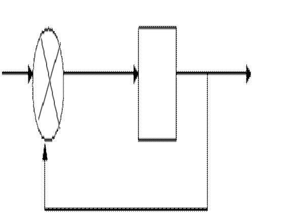
Consider the closed loop system shown below whose G (s)= k(s+2) / S2 + 6*s+10

The gain k is to be varied.
The root locus plot of G (s) is obtained by using root locus command as illustrated below
% Root locus for G(s) = (s+2) / (s*s+6*s+10)
clf
num= [1,2];
den = [1 6 10];
rlocus(num, den);
Execution of the above program yields the following root locus.
After the above display, if the following is typed>>[k,Poles]=rlocfind
(num, den) and the cross hair cursor is moved by means the mouse to any
point on the root locus, Clicking the mouse at that point displays the
value of k and location of all closed loop poles corresponding to that
value of k.
Customizing here refers to changing the scale of the plot along the real and imaginary axis. So that the desired region can be seen more clearly leaving the unwanted part. The following third order system illustrates the use of axis command to achieve the above.
% Root locus of a thrid order system
clf;
num=1;
den=conv([1 20],conv([1 0],[1 1]));
rlocus (num,den)
The system has no zeros and three poles at 0, -1 and –20. Execution of the above yields the following root locus.
If the effect of pole at – 20 is ignore and concentration is around origin, it is difficult to see the plot clearly. For seeing the Plot more clearly the portion of the locus corresponding to dominant Poles (i.e) around origin, customization of the graph is done.
The following Program illustrates this
% Customization of Root locus
clf
num=1;
den=conv( [1 20],conv ( [1 0] , [1 1] ));
rlocus (num,den);
axis ( [-2 2 – 6 6 ] )
This axis command plots the Root locus with the desired formatting and is shown below
The gain at which the system becomes unstable can be easily found from
the above from the crossover points of Imaginary axis.
Root locus plots can be used as effective design tools for controller design. This is illustrated below for designing a controller for a plant.
G (s)= 1/ [s (s+1) (0.2s+1)]
Three types of controllers are considered a pure gain controller, a lead compensator and a lead lag compensator. The specifications are that the closed loop system should have a damping ratio of 0.707 and largest possible natural frequency.
For the design of pure gain controller the root locus is plotted as such and is as shown below. The plot is expanded in the region of interest. The pole at s= -5 decreases to –µ and hence ignored. The command sgird super impose a 45[A1]° line corresponding to damping ratio of 0.707 an+d dotted curves corresponding to natural frequencies of 1, 2, 3 and 4 rad/sec on the plot.
The program and the plot are given below
% Design by means of root locus
clf
num=|;
den=conv( conv([1 0], [1 1] ), [0.2 1 ] );
rlocus (num,den);
vl = 0.1;
v2=2.5;
hl = 4;
h2 = 0.1;
axis ([-h1 h2 – v1 v2]);
damping = 0.707;
wn= 1:1:4;
sgird ( damping, wn)
Execution of the above program yields the following plot
As seen from the Plots, the pure gain controller achieves a damping coefft of 0.707 at a natural frequency of approximately ½. The corresponding gain K=0.41 which is found by using the command [k, poles] = rlocfind ( num, den) and clicking on the graph at the intersection point of 0.707 damping.
The command sgrid without any arguments super imposes a grid on an existing root locus plots with ten lines of constant damping ratio equally spaced from 0.1 to 1.0 and lines of constant natural frequency.
3.2 LEAD COMPERNSATOR:
Adding a lead compensator is another standard way of improving the natural frequency of the closed loops system. For a system with three real poles, the zero of the compensator is placed closed to the middle pole. The pole of the compensator is placed as far to the left as possible, normally ten times the compensator zero.
The lead compensator is chosen as K (S+1) / (1+0.1S)
The corresponding root locus is created and superimposed on the previous example by running the following program.
% adding a lead compensator
hold on
num = [ 1 1];
den = conv(conv(conv([1 0],[1 1]), [0.2 1 ]), [0.1 1 ]);
rlocus (num, den)
hold off
The plot is a line leaving the real axis at s= -2.
For achieving a damping ratio of 0.707, the gain K = 1.64 and Wn = 2.7
3.3 LAG COMPENSATOR:
The steady state performance of the closed loop system can be improved without significantly reducing natural frequency by adding a lag compensator.
The compensator pole is chosen close to origin at – 0.005.
The zero is chosen at – 0.05
The lead lag compensator is {K (S+1)(20S+1) / (0.1S+1) (200S+1)
The lag compensator has slightly decreased Wn, but the steady state error is decreased, since the gain K corresponding to danping ratio 0.707 is 16.35. With only lead compensator the steady state error for a unit ramp input is 0.6 where as with lag compensator added it is 0.06.
The frequency response and stability analysis can be done for a system whose transfer function is given. The following program illustrates the same for a transfer function.
%Creating root locus, bode plot, nyquist plot
% and nichols chart for the following transfunction
num = 18*[1 20];
den =conv(conv([1 15],[1 25]),[1 0.4]);
sys1 = tf(18*[1 20],conv(conv([1 15],[1 25]),[1 0.4]));
%impulse(sys1,'r')
sys2 = frd(10,20);
subplot(2,2,1)
rlocus(num,den)
%rltool(sys1)
%rlocfind(sys1)
%sgrid(sys1)
%zgrid(sys1)
subplot(2,2,2)
%bode(num,den)
margin(num,den);
subplot(2,2,3)
nyquist(num,den)
subplot(2,2,4)
ngrid('new')
subplot(2,2,4)
nichols(num,den)
The corresponding plots are shown here: